Reprinted with permission from the author Roger Delpech and the publication School Science Review.
School Science Review (the ASE’s journal for science education 11 – 19), ASE, March 2006, 87 (320)
Abstract
This paper introduces the use of a gaseous CO2 sensor and data logging equipment, for a variety of purposes in the school laboratory, including measurements of respiratory and photosynthetic rates of animals, plants and microbes. Suggestions are made for taking measurements in the field, as well as demonstrations and project work in the school laboratory. A simple equation for converting rates of change of gaseous CO2 concentration change into energy or glucose equivalents is suggested.
Introduction
Most people have fantasized about what it would be like to be invisible to others. This paper concerns the opposite – making an otherwise invisible gas, carbon dioxide, visible (at least in a quantitative sense). This is now something that can be achieved, at a realistic cost, in the school classroom, due to the production of a gaseous CO2 sensor by the USA based company Vernier [Software & Technology] (distributed in UK by Instruments Direct Ltd).
There is growing consensus amongst scientists that the world is going through a period of rapid climatic change, driven at least partly as a result of anthropogenic production of greenhouse gases such as CO2 (Maslin M 2004). The complexity of these issues has the effect of reducing pupil interest, partly because they cannot see the immediate relevance of climate change to their own lives, and partly because they cannot see what impact their lifestyle choices (ecological footprint) might have on the global picture. Historically, climate change has always had a powerful effect on human affairs, as brilliantly described by Brian Fagan (Fagan 2004), and the recent catastrophic effects of hurricane Katrina in the southern USA shows that modern humanity is even more at risk, despite technological advances. Global warming is a key topic in most GCSE and A-Level Biology specifications, and new Edexcel Salters Nuffield AS Biology course includes a significant section on plants and climate change (Salters 2005) where pupils are asked evaluate evidence.
Most school pupils will have been introduced to the critical role of photosynthesizing plants in removing CO2 from the atmosphere as part of the carbon cycle, and the release oxygen as a waste gas. Even though the importance of learning these cycles is emphasized, it is normal for students to be expected to accept the details on trust.
Standing outside the classroom, in a green environment, it is simply not possible to actually see the carbon dioxide being taken up by the leaves of the plants, or released by the decomposers in the soil – but now there is technology that allows us to monitor what is going on, and even calculate some of the figures involved.
A fantasy series of lessons on the carbon cycle
This could be used at any level, and would make photosynthesis, and responsible citizenship in relation to ecological footprints, seem very personally important to each individual pupil.
Everybody fears suffocation – re-breathing air into an empty bag is only possible for a moment – chemoreceptors lining blood vessels leading to the brain instantly detect rising levels of bicarbonate ions in the blood and within moments, we are tearing the bag from our face, and gulping fresh air. It is the rising CO2 levels in the blood which trigger changes in heart and lung activity during exercise, not falling O2 levels.
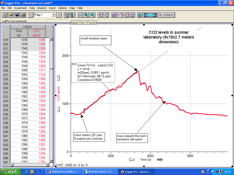
Imagine a lesson that begins with a class entering a laboratory. They notice the windows have been closed, even though the day might be warm (if plants are present, they should be covered with black plastic bin-liners). On a screen there is a display provided by a data-projector linked to the CO2 probe and LabPro, showing a scrolling graph of the CO2 level in the room plotted against time. Once the door is closed and the class settled down, they notice the rising level of CO2 on the display.
It is the mixing of CO2 expelled on the breath of the teacher and pupils, with the air in the room, which will cause the graph to rise, and the gradient of the graph will provide a rate. This gradient can be instantly found using a tool button on the graph screen (see instructions of the use of Logger Pro 3 software later) – which gives the rate of change in parts per million (ppm) per second. This rather academic figure can be converted by a simple calculation to equivalent units of glucose or energy (see Box 1)
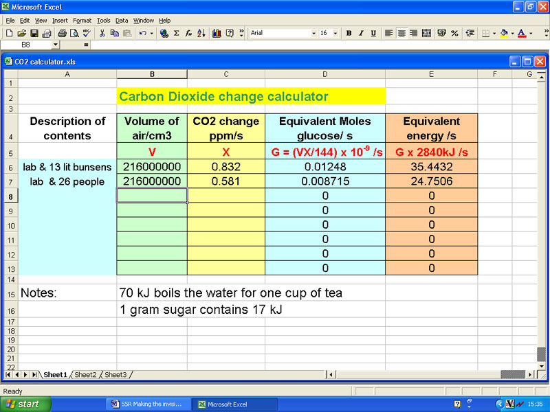
Box 1 – Calculations based on rates of change in CO2 concentration
If the rate of CO2 uptake or production is known, then it can provide a means for calculating the equivalent number of glucose molecules that this amount of CO2 represents, either being made during photosynthesis, or broken down during respiration. If this assumption is made, then it is possible to estimate the amounts of energy being used in photosynthesis or released in respiration.
Select an area of the graph, and select the rate button to get the rate of CO2 change figure for this region. The software provides units for the rate of CO2 change in ppm/second.
This rate of change in CO2 would be different for different sized containers, so the next step is to taken account of the volume of gas in the container being used, in units of cm3.
If we assume that six CO2 molecules are (used in photosynthesis to form/are released by the respiration of) a glucose molecule, then the number of moles glucose being formed per second =
(Rate of change (ppm) x Volume of container (cm3) / 144 ) x 10-9
The complete aerobic respiration of glucose is worth 2840 kJ / mole. So the rate of release of energy (or uptake of energy in photosynthesis) by the organism in kJ per second =
(moles glucose per second) x 2840 kJ.
For many purposes, it would be a good idea to have an Excel worksheet set up so that simply entering the volume of the container, and the ppm/second figure, leads to the automatic calculation of glucose and energy equivalents.
Naturally this figure can be adjusted to provide a rate in kJ per minute, per hour, or per day! To allow fair comparisons between different samples, the figure should also be related to the mass of biological material involved, to provide a rate as units of energy/unit mass/unit time.
For even more drama, the Bunsen burners in the laboratory could be lit for a ten minute period, and the change in the gradient of the graph will soon be apparent (a nice parallel with fossil fuel combustion and the composition of the global atmosphere).
The burners are turned off, and the windows opened to allow fresh air to circulate the room, and to vent the CO2 – this can be followed on the scrolling graph (see screen shot 1). Incidentally, building regulations recommend the CO2 levels in rooms are kept below 1000 ppm, however it is commonplace for stuffy teaching rooms to have levels as high as 4000 ppm!
Screen Shot 1

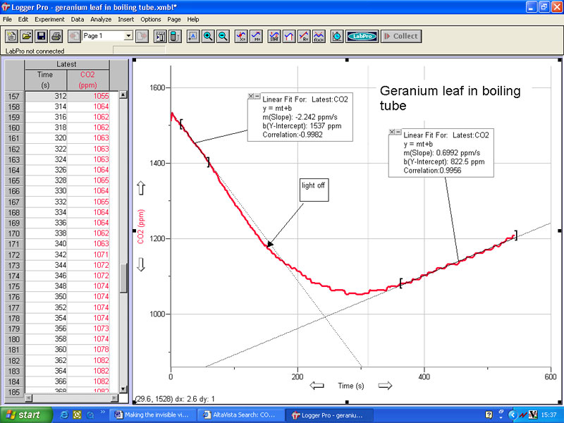
The CO2 probe is then placed in a [test] tube with a freshly detached plant leaf, covered by a lightproof sleeve (lightproof card or aluminum foil). The first surprise for many pupils is to see that the leaf in the dark is doing what we do – creating CO2 rather than taking it up; this provides an opportunity to recognize that respiration is a universal feature of living organisms. Then the sleeve is removed and a bright light shone on the tube…and within a couple of minutes, the CO2 levels will begin to fall (thunderous applause from the class!). The advantage of using a single leaf in such a small container is that the change in carbon input/output will be seen in a couple of minutes (screen shot 2).
Screen Shot 2
The lesson finishes with an attempt to estimate the number of such illuminated leaves that would be needed to stabilize the CO2 levels in the lab – by balancing the CO2 output of the class with photosynthetic uptake of CO2 by plant leaves. Guidance with the calculations are found in boxes 1 & 2.
Box 2 – Calculating the need for plant leaves to reprocess an individuals CO2, and replenish the oxygen consumed in respiration
Find the volume of the laboratory by multiplying its length, breadth and height in meters, and then multiplying the answer by 106 to give its volume in cm3.
Assume that the gradient of the CO2 increase in the laboratory, with the doors and windows closed (and plants covered), is largely due to the respiration of the humans in the room, and use the formula below to calculate the number of moles glucose being respired per second by the humans present:
(Rate of change (ppm per second) x Volume of container (cm3) / 144) x 10-9
Divide this figure by the number of people in the room, to find out the number of moles of glucose per second being respired by each person.
Assume that the leaf in the boiling tube is in volume of 50 cm3 of air, employ the formula above to calculate the number of moles of glucose per second being made in the tube when the leaf is photosynthesizing in the light – this is the net productivity** of the leaf, due to the fact that the leaf has to both make the glucose to pay off its respiratory needs, before it actually makes a “net profit” of extra glucose for use in growth etc. This net productivity is what is needed to reprocess the CO2 released on an individual’s breath, back to O2.
Divide the figure for the CO2 output of an individual, by the figure for the CO2 uptake by an illuminated plant leaf, and the answer gives the number of illuminated leaves that would be essential to reprocess the exhaled carbon dioxide of an individual student.
A sobering thought for students is that plant leaves are only naturally illuminated for half of the 24 hour day/night cycle, and that climatic conditions, seasons, disease and many other factors will reduce further the capacity of a leaf to help us breath in this way! In addition, the draughtiness of the room will mean that the values for class respiration will be significantly less than the textbook values.
**To find the gross productivity of the leaf, employ the formula above to calculate the number of moles of glucose per second being respired by the plant leaf in darkness (because this is still happening when the leaf is in the light). The gross productivity of the leaf is the sum of this figure plus the net productivity figure.
Future lessons might involve going into the garden or field to measure the real inputs/outputs of CO2 by plant leaves, the soil, and small invertebrates. The rest of this paper describes the probe and a range of ways in which the CO2 probe can be adapted for these purposes. Further suggestions and details can be found on the SAPS website (www.saps.org.uk).
The principle upon which the CO2 probe depends
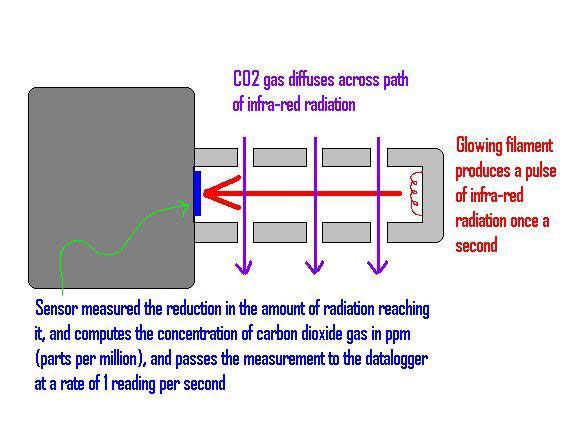
Figure 1
The sensor depends on the fact that gaseous CO2 intercepts pulses of infra-red radiation produced by a filament at the end of the sensor probe; the more CO2 there is in the air, the less radiation reaches the infra-red sensor (see figure 1). This, of course, is the basis for the greenhouse gas effect; where the heat that should be radiated to outer-space from Earth is hindered from doing so by greenhouse gases such as CO2 and methane. So discussing the function of the probe can actually form a useful basis for understanding the greenhouse gas effect.
What are the advantages of using a gaseous CO2 sensor, as opposed to a gaseous or aqueous O2 sensor?
Gaseous diffusion is thousands of times faster than diffusion in water, allowing results in minutes rather than hours (allowing time for replications and modifications). There is much less CO2 as a fraction of the atmosphere, so changes are more obvious, allowing results to be obtained in minutes rather than hours (and by using small container volumes, only small amounts of biological materials are needed). No difficult experimental concepts are required to understand the fate of the CO2 in photosynthesis – what you see is what you get. The analogy between the principle on which the probe works (see figure 1), and global warming, can be explored. Used with a laptop, the Vernier software allows dramatic real-time plotting and annotation of data whilst it is being collected, as well as sophisticated analysis tools. The [LabPro] can be used on its own and the data downloaded later, or with a [Texas Instruments graphing calculator] to provide a current display.
A range of possible methods for employing the CO2 probe
Probe placed in 250 cm3 bottle (supplied with kit)
This can be used with either animal and plant material, or both animal and plant material, to show the evolution and uptake of CO2. If both sorts of material are present, it might be possible to achieve a balance (by varying the size, or species of a leaf, or the intensity of light provided). Placing animals and plants together and achieving a balance of input and output of CO2 has obvious parallels with the problems of achieving CO2 stability in the atmosphere of the world today. Important ecological messages should be loud and clear after such classroom activities.
A single bee or hoverfly might be persuaded to spend some time flying in such a bottle, so that the extra cost of such locomotion can be judged by the increase in CO2 output during periods of flight. Use a bee, a beetle, woodlouse, snail, stick insect, earthworm, large spider or moth- they all work well! The sensitivity of the system is such that ventilation patterns for an individual animal can be distinguished; for example a bee and an earthworm seem to continuously exchange gas with their environment, whereas a housefly seems to breathe in a more cyclic manner, closing its spiracles between ventilation movements. A garden spider shows the same cyclical ventilation patterns. A bumblebee can show that after being fed with a drop of sugar solution, its metabolic rate increases. These observations would enliven any lesson dealing with the process of gas exchange between animals and their environment.
A significant point to note is that the orientation of the bottle should be kept the same when recordings are made, as CO2 will concentrate slightly in the lower regions of the vessel.
Probe placed in a [test] tube
A substitute rubber [stopper] must be created for allowing the probe to be used in a [test] tube, and is illustrated by [the] figure [at the right]. This will provide a gas-proof seal between probe and the air in the boiling tube.
The small air volume in the tube means that the response time will be as fast as possible. Very small animals are perhaps best studied in such a small chamber to increase the speed of result collection, and a leaf can be rolled so that it sits such a tube. The tubes can also be easily illuminated or warmed or cooled in a water bath, to study the effects of light intensity or wavelength (wrap coloured sheets of cellophane around the tube) or temperature on photosynthesis.
Small samples of soil can be placed in the tube, in order to measure the overall respiratory activity of the decomposers present – a major way in which carbon is recycled to the atmosphere. Of course, these soil samples can be modified by the additions of solutions of water, acids, lime, pesticides fertilisers, etc. in order to see the effects of such additions on the respiratory activities of the soil microbes.
Alternatively, a few cm3 of a solution containing microbes, such as soil water, pond water, or yeast cells in a sugar solution, or non-sterilised milk, or bacteria growing in nutrient broth, seem to produce CO2 at steady rate that reflects the total populations of microbes.
Probe placed in a bell-jar
For larger creatures such as whole potted plants, a bell-jar placed on a glass sheet should provide a useful container. With an air volume of several liters, the response time for the set-up will be slower than that for the smaller vessels, and if soil microbes are to be kept out of the equation, then the plant’s pot of soil should be wrapped in plastic. It will give pupils a new appreciation of the value of potted plants on windowsills!
Probe placed in a plastic bottomless [soda] bottle
This apparatus is useful for studying the carbon budget of patches of ground vegetation, and underlying soil, by simply pressing the bottom of the [bottle] onto the ground. As long as the base is pressed firmly onto the soil in order to create a seal. This has been used to compare sunlit patches of a lawn, with patches in the shade, and with bare soil. A brightly lit piece of a lawn will be a net importer of CO2, whereas a part of the lawn in the shade may well be a net exporter, because the rate of photosynthesis in the grass leaves is not sufficient to exceed the respiration of the grass plants, their roots and the soil organisms.
Probe placed in a bottomless plastic bottle, with a plastic bag sealed to its base
This can be used to isolate individual leaves or small branches on taller above ground vegetation in order to study the carbon budget of the leaves still attached to the plant in the field. Larger and smaller clear plastic bottles can be adapted by cutting the necks in the appropriate place. This gives a fairly consistent volume of air surrounding the leaf. The plastic bag can be gathered up like a skirt, and stuck with tape, to form a reasonably CO2 proof seal on the branch. Alternatively home-made frames of fixed volumes could be made, using sheets of plastic and tape. Direct collection of CO2 data from living plants in the field will make the whole concept of the carbon cycle much less a question of trust.
Probe placed in a metal sleeve, already pushed into the soil
This enables the collection of CO2 produced by the respiration of soil organisms. A simple steel cylinder (diameter 30 mm x length 150 mm) fits the probe + [stopper]. The metal sleeve can be driven say 10 mm into the soil, thus providing a finite soil area for CO2 sampling, before the probe is attached. Within a few minutes a trace of the CO2 output of the soil will be obtained. An alternative is to collect soil samples, and carry out the measurements in [test] tubes, back in the laboratory – this would have the advantage of allowing varying amounts of water, pH buffers etc. to be added in order to assess the effects of soil moisture, pH etc. on respiratory rates of decomposers. The respiratory rates of different kinds of soils and types of leaf litter, or by excavating a hole, different soil horizons, can be compared. This tool is particularly robust and can be easily cleaned for re-use.
A large proportion of the world’s organic carbon is present in the soil as organic detritus, and the respiration of soil detritivores and decomposers releases a significant proportion of CO2 back into the atmosphere. The warming of Polar Regions, including regions of permafrost where much of the world’s peat is currently locked up in the ice, could lead to an accelerating greenhouse effect, as the trapped carbon is respired. Experimental studies on soil and peat respiration are currently highly relevant to this potential problem.
Using the Vernier CO2 sensor, [LabPro] data logger, and Logger Pro 3 software to collect and analyse data
A very strong reason for using the Vernier data logging system is the exceptional quality of the Logger Pro 3 software that comes with it, and comes with site and student licence. The following instructions give an idea of the employment of the software with the CO2 sensor:
Make sure all cables between sensor, [LabPro] data logger, and computer are attached, and that the data logger is powered up. Then, when you start the Logger Pro 3 software running, it will recognise which probe is attached and will provide you with a blank graph already bearing the correct axes (time /secs on the x-axis, and CO2 level/ppm on the y-axis). At this stage, even before you collect any data, there will be a glow at the tip of the probe, about once every second, as it begins to register CO2 levels.
To start collecting data, simply select the Collect button on the tool-bar at the top of the screen. The graph should immediately show data being collected. You can stop collecting at any point in time by clicking on the Stop Collecting button. It is worth bearing in mind that there is a warm up time of approximately 90 secs before the data makes much sense.
The usual default time for collecting is 300 secs, but if you want to extend this time (which can be done whilst data is being collected), click on Experiment and then select Extend collection from the drop down menu. If you wish to extend further, just keep selecting the same drop-down option
The scrolling columns on the left of the screen will show the numerical values of the readings as they are being taken.
One of the most exciting aspects of this data logging kit is that you can enhance your view of the data as it is being collected by stretching or shrinking either or both the x and y axis of the graph.
To do this move the cursor to just outside the border of the axis you wish to change (it will show a sort of squiggly line), and then right click and drag away from the origin of the axis, or towards the origin of the axis, to stretch or shrink the axis of the graph, respectively.
Don’t worry if you have lost the scrolling data, you can move to where you want on the graph, by clicking on the direction arrows, found either side of the title for each axis.
In this way you will be able to enlarge any portion of the developing graph to increase its dramatic impact!
One of the delights of the Vernier software is the ability to add labels, titles and other features to the graph – even when data is still being collected. The most immediately useful analysis feature is the gradient function, which will get the software to calculate the slope of a best fit line between any two points on the graph; and you can identify different parts of the graph for separate analysis:
Simply highlight the portion of the graph you wish to study by clicking and dragging the cursor so that the area of interest becomes highlighted, and then click the Linear Fit (R=) button on the toolbar at the top of the page. A box will appear on the page which indicates the slope, as well as providing a correlation coefficient for the data in the regions of interest. This box can be dragged to wherever it seems most appropriate on the page (if data is still being collected, the calculation will not be completed, until the data collection stops).
If you select the Stop Collecting data button, then you can save the file if you so wish. When you select Start Collecting data again, the program will ask you if you want to erase the current data, or append the new data to the previous set. Normally you will want to start with a “clean sheet”, but occasionally you may wish to leave the previous trace on screen and run the new trace over the same area of the graph; in this case you should select Experiment….Store latest run. Then you can start to collect a new set of data, with the previous trace on screen in the background.
Acknowledgements:
The author wishes to thank Dr Mike Lexton for advice on the calculations for this paper, as well as Harpreet Aluwahlia for technical assistance. In addition he would like to express his gratitude to Paul Beaumont of SAPS, and the Trustees of the Gatsby Charitable Trust whose generous support has been essential.
References:
Diamond Jared Collapse
Fagan Brian 2004 The long summer: how climate changed civilization Granta ISBN 1 86207 644 8
Maslin Mark 2004 Global Warming: A Very Short Introduction OUP ISBN 0-19-284097-5
Salters 2005 Salters Nuffield Advanced Biology AS Heinemann ISBN 0 435 62857 7
Box 3 – Suggested investigations using the CO2 sensor
These suggestions go well beyond the scope of fieldwork, but should give some idea of the range of uses to which the CO2 probe might be applied.
Effects of the following on leaf photosynthesis:
- CO2 concentration
- temperature
- light intensity
- light wavelength
- daily rhythms
- stomatal density
- light/dark leaf adaptations
- herbivory
- action of herbicides
- C4 & CAM versus C3 plant leaves
Effects of the following on teaching room gaseous CO2 concentrations:
- Air-flow through the room
- number of people in the room
- biomass of people in the room
- physical activity in the room (compare a day when everyone is doing test, with another day)
- size of the room
- combustion sources of CO2 (Bunsen burners)
- presence of plants
Isolate the different parts of a shrub in the field to study the carbon budget:
- in different aspects (shade adapted leaves v light adapted leaves)
- at different times of the day
- in different weathers
- at different times of the year
Study the carbon budgets of germinating seeds, and follow their carbon budgets:
- as they grow into seedlings with leaves
- metabolic rates of fruits can be studied during the ripening process
Isolate the carbon budget of plant roots and associated soil, from the above ground carbon budget (with a potted plant)
- investments in shoots/roots when grown at different angles
- when mechanically stimulated/stressed
Effects of the following on respiration of small invertebrates:
- Temperature
- Activity (walking/flying)
- food sources
- stage of development
- species
Effects of the following on soil respiration:
- moisture content
- % organic matter
- temperature
- pH
- litter type
- mineral content
- mineral skeleton
- supplements of nutrients
- living plants
- organic & inorganic fertilizers
- pesticides
- salinity
- acid rain
- soil invertebrate population
- microbial populations
- season
- weather
Effects of the following on microbial cultures in liquid media (yeasts, bacteria):
- Types of C-source
- Concentrations of nutrients
- age of culture
- age of fermentation
- pH
- salinity
- mineral supply
- microbiocides
- ethanol content
Effects of the following on microbial populations in milk and dairy products:
- Temperature and growth of spoilage microbes
- temperature and growth of lactic acid bacteria
- species of bacteria
- temperature and pasteurisation/sterilisation
- sources of milk
- process of yogurt production
- size of starter culture
- effects of pH
- effects of additions of lactic acid