In Vernier Video Analysis, velocity is calculated using a numerical derivative. The default calculation uses seven points, three on either side of the position point of interest, to calculate the object’s velocity at the point of interest (for additional details, see https://www.vernier.com/til/1011). While useful for reducing the effect of point-marking inconsistencies, the calculation is problematic when changes in position happen rapidly, such as when an object collides with another object. Often in such situations, the goal is to determine the velocity of the object just before or just after the collision. However, the numerical derivative calculation provides a poor estimate for the velocity in which you are interested.
Figure 1 shows typical data for a bouncing ball. As expected for an object in freefall, the velocity appears linear while the ball is in the air. The velocity values do not follow this pattern at the bounce point because the velocity calculations use position data from both sides of the bounce. The number of velocity points affected (i.e., they don’t follow the linear pattern) is directly related to the number of points used in the numerical derivative calculation.

What follows are three options for obtaining a more accurate estimate of velocity for situations in which position changes rapidly, such as a bouncing ball. Not every method will work in every situation, so you will want to select the method that works best for your data.
1. Adjust the Number of Points in the Velocity Calculation
A custom calculated column can be used to calculate velocity using fewer than the default seven points. Follow these steps to create the calculated column:
- Click or tap Columns Options,
 , for any column in the data table, and select Add a Calculated Column.
 - Enter a Name and Units for your column.
- Click or tap Insert Expression and select Custom Expression.
- Enter the expression firstDerivative(Y, X, n) where Y is the position column, X is the time column, and n is the number of points used in the derivative calculation. Follow these guidelines when entering the expression:
- Data column names must be in quotes (e.g., “Y” and “Time”).
- Supported values for n are 3, 5, 7, 9, 11, 15, 21, 29, 39, 51, 65, 81, and 97.
- If n is not specified, the default value of 7 is used.
- Figure 2 shows the expression used for velocity calculations for y position data using three points.

- Click or tap Apply.
Figure 3 shows a comparison between the 3-point and 7-point velocity calculations. While there is some variation in measurements over the entire motion, the most noticeable differences come for the points around the bounces.

For the bouncing ball, the 3-point velocity calculation provides a better estimate for the velocity just before and just after the bounce. However, it does not completely resolve the issue. Additionally, the 3-point method makes all velocity measurements more susceptible to inaccuracies from mismarked position points. The following calculation methods address these concerns.
2. Mark the Motion using Multiple Objects
One way to remove the dependence of the velocity measurement on points before and after the bounce is to mark the points in separate sections using the Vernier Video Analysis Objects feature, . Follow the instructions below to mark sections of your motion using multiple objects.
- Review the motion of your object(s) and decide which sections of the motion should be marked using separate objects. For the bouncing ball data, the motion can be separated into three sections: the motion before the first bounce, the motion between the first and second bounces, and the motion after the second bounce (see Figure 4.)
- Mark the data points as you normally would for the first section of your video.
- Once that is done, click or tap Objects,
, and select +ADD NEW OBJECT.
- Now mark points for the second section of your video.
- Repeat Steps 3 and 4 until you have marked all sections of the video.

Figure 5 shows a comparison between the velocity values calculated using the entire motion as a single object (Y Velocity) and the same motion captured using three separate objects. The default 7-point velocity calculation was used for all objects.

Around the bounce, the velocity estimates for the separate objects are much better than the estimates you get with the motion captured using a single object. Notice that this method does not affect velocity measurements away from the bounces.
This method can be used along with the 3-point velocity calculation; however, you would need to add a calculated column for each section of your motion since the position data for each section are in separate data columns.
3. Model the Velocity Data
If your velocity data follow a known model, you can apply a curve fit to estimate the velocity values near the bounce points. Follow the instructions below to use a curve fit model to estimate velocity.
- Click-and-drag or touch-and-drag across the graph to select the portion of the velocity graph you want to model.
- Click or tap Graph Tools,
, and select Apply Curve Fit.
- Select the desired curve fit model, then click or tap Apply. For the bouncing ball data, the curve fit model would be Linear.
- Click or tap Graph Tools,
, and select Interpolate. When Interpolate is selected, the value of the model at the selected x coordinate is shown.
- Click or tap anywhere on your graph to display the Examine line.
- Drag the Examine line to your desired point on the graph to view the model’s estimate for velocity at the desired point.
- Repeat this process for other sections of your data that you need to model.
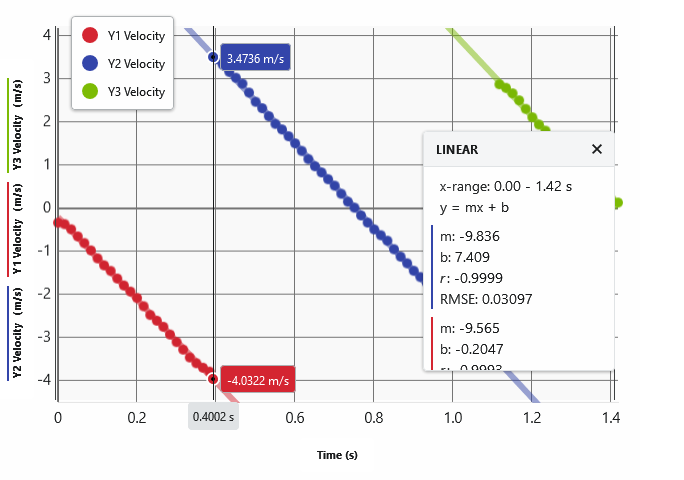
Figure 6 shows velocity estimates using linear models at the time the ball was on the ground as shown in the video (see Figure 1). While it may seem reasonable to use these values, it is impossible to know the exact time at which the ball first struck (or later left) the ground unless that information is shown explicitly in the video. Thus, it is best to use the time associated with the last data point before the bounce (and the first data point after the bounce) when using a curve fit model to estimate velocity.
For additional information on using the Vernier Video Analysis App, see
Vernier Video Analysis Troubleshooting and FAQs