Sharing ideas and inspiration for engagement, inclusion, and excellence in STEM
Beer’s law is a cornerstone of high school and introductory college chemistry—but it’s often taught with chemicals that require extra safety considerations and disposal planning. After teaching Beer’s law for decades using traditional compounds, I’ve found that food dyes and sports drinks offer a practical alternative that keeps the focus where it belongs: on student data and sensemaking.
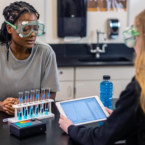
In this investigation, students use spectroscopy to analyze food dye concentrations in popular sports drinks. They collect full-spectrum data, compare transmittance and absorbance, build a Beer’s law calibration curve, and apply it to determine an unknown concentration—all using a green chemistry approach that still produces excellent results. This instructional sequence was developed with my colleague Dr. Melissa Hill, who adapted an AP-style transmittance–absorbance comparison for a Beer’s law investigation that works across chemistry courses.
Using Spectroscopy to Answer a Real-World Chemistry Question
Students use a spectrophotometer to determine the concentration of Blue Food Dye #1 in a sports drink by applying Beer’s law. Rather than starting with an equation, the lab is framed around a concrete question students can reason through, “How could you determine how much food dye you ingest when you drink a 16-oz sports drink?”
To answer it, students investigate:
- How light interacts with colored solutions
- The difference between transmittance and absorbance
- Why absorbance changes linearly with concentration
- How a calibration curve can be used to determine an unknown
This question-driven approach helps Beer’s law emerge naturally from the data, rather than feeling like a formula students are asked to memorize.
AP Chemistry Connection
The transmittance-to-absorbance comparison mirrors the data reasoning emphasized in AP Chemistry—particularly how %T and absorbance are related—before extending that reasoning into a full Beer’s law application.
What You’ll Need
- Go Direct® SpectroVis® Plus Spectrophotometer
- Devices with our free Vernier Spectral Analysis® app
- FD&C Blue #1 food dye stock solution (~50 mL per lab group)
- Distilled water
- Eyedroppers
- Clear plastic cuvettes
- 10 mL graduated cylinders
- Sports drinks with Blue #1 food dye
- Plastic Beral pipets or eyedropper
- Test tubes and racks
Tech Tip
For quantitative spectroscopy, aim for solution absorbance values between ~0.1 and 1.0 AU. This range produces the most reliable data and avoids sensor saturation.
Preparing the Stock Dye Solution (Teacher Prep)
Before class, prepare a stock solution of blue food dye for students to dilute. After years of trial and error, I’ve found the most reliable approach is to check absorbance first, then adjust concentration as needed.
- Add a few drops of blue food coloring to several hundred milliliters of water.
- Mix thoroughly.
- Measure the absorbance using the spectrophotometer.
- Dilute or add dye until the absorbance at the peak wavelength is close to ~0.9 AU.
Because food dye is inexpensive and nonhazardous, precision at this stage doesn’t need to be perfect—students will still generate strong, meaningful graphs.
Pre-Lab Analysis: Preparing Dilutions for Beer’s Law
Before students prepare their Beer’s law dilutions, the pre-lab asks them to connect the structure of FD&C Blue #1 to its color and solubility, think through how a spectrophotometer measures light, and calculate the concentrations they’ll need—so when they begin mixing solutions, they already understand what they’re making and why.
With that groundwork in place, students are ready to prepare the dilution series that will be used to generate a Beer’s law calibration curve.
Students prepare a series of 10 mL dilutions from the Blue #1 stock solution to create known concentrations that span an appropriate range for spectrophotometric analysis.
| Table 1 | |||
| Blue #1 solution test tube | Blue #1 stock solution (mL) | Distilled H20 (mL) | [Blue #1] (M) |
| 1 | 10 | 0 | 5.85 × 10⁻⁶ |
| 2 | 8 | 2 | 4.68 × 10⁻⁶ |
| 3 | 6 | 4 | 3.51 × 10⁻⁶ |
| 4 | 4 | 6 | 2.34 × 10⁻⁶ |
| 5 | 3 | 7 | 1.75 × 10⁻⁶ |
| 6 | 2 | 8 | 11.7 × 10⁻⁶ |
| 7 | 1 | 9 | 5.85 × 10⁻⁷ |
| 8 | 0 | 10 | 0.00 |
Example table with calculations based on the concentration of the Blue #1 stock solution = 5.85 × 10⁻⁶ M
Part 1: Exploring Transmittance and Absorbance
Students begin by examining how light interacts with their, most concentrated sample.
Calibrate the Spectrometer
- Launch Spectral Analysis and connect the Go Direct SpectroVis Plus Spectrophotometer.
- Select Advanced Full Spectrum mode.
- Calibrate using distilled water as the blank.
Measure Transmittance
- Switch to Transmittance mode.
- Insert the stock dye solution.
- Observe which wavelengths pass through the solution.
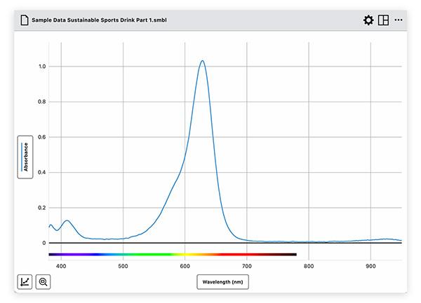
Switch to Absorbance
- Change the measurement mode to Absorbance.
- Compare the absorbance spectrum to the transmittance data.
For many students, transmittance is not immediately intuitive. One helpful connection is that our eyes are transmittance detectors—we only see light that reaches them. Regions of low transmittance correspond to wavelengths absorbed by the dye, often in the yellow-orange region for Blue #1, while higher transmittance in the blue region explains the solution’s color.
Part 2: Investigating the Effect of Concentration on Light Absorption
Students investigate how transmittance changes as concentration increases.
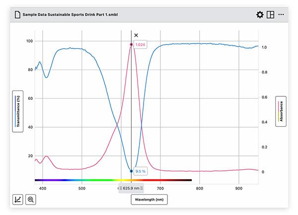
Data Collection: Transmittance vs. Concentration
- Set the spectrophotometer to Transmittance vs. Concentration.
- Select the wavelength corresponding to the minimum transmittance (λmin).
- Measure each dilution using event-based data collection.
As students graph the results, they observe that transmittance decreases non-linearly as concentration increases.
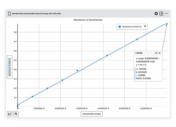
Data Collection: Absorbance vs. Concentration (Beer’s Law)
Next, students repeat the process using absorbance.
- Switch to Absorbance vs. Concentration.
- Select the wavelength of maximum absorbance (λmax).
- Measure absorbance for each dilution.
Part 3: Relationship Between Transmittance and Absorbance
Once students have graphed both percent transmittance and absorbance against concentration, they compare the trends. The %T graph curves, while the absorbance graph is linear and easier to interpret.
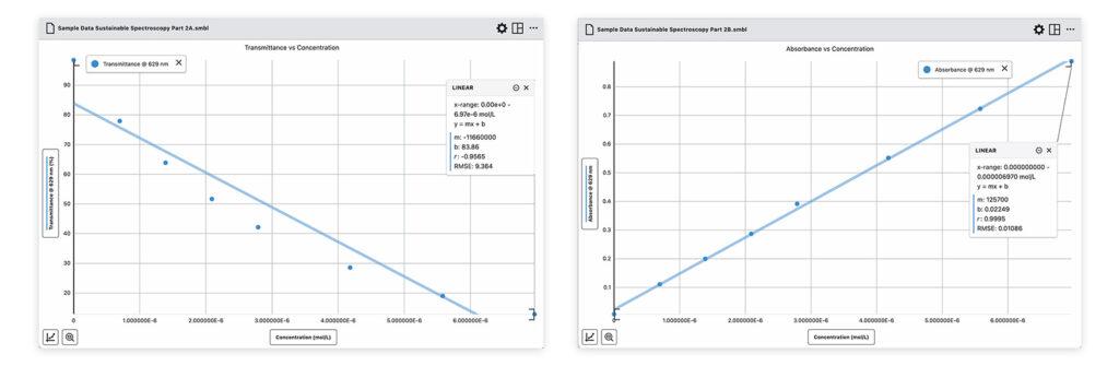
At this point, students are introduced to the mathematical relationship between transmittance and absorbance and asked to consider how that equation explains the shapes of their graphs. With that connection in place, they revisit their absorbance vs. concentration data and see why Beer’s law works so well—when wavelength and path length are held constant, absorbance is directly proportional to concentration.
Part 4: Determining the Dye Concentration in Sports Drinks
With a Beer’s law curve established, students are ready to analyze real sports drinks.
Students begin by measuring the absorbance of an unknown sports drink sample at the selected wavelength (λmax). Because absorbance has already been shown to vary linearly with concentration, this single measurement can be used to determine the dye concentration.
Students then use one of two approaches—both supported in Spectral Analysis—to find the concentration of Blue #1 in the drink
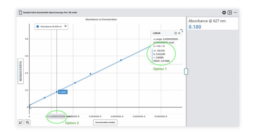
Option 1: Use the linear fit equation from their calibration curve and solve for concentration. Students treat the absorbance of the sports drink as the y-value and solve the linear equation for x (concentration).
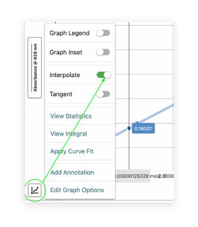
Option 2: Use interpolation tools in Spectral Analysis to automatically determine the concentration value. Students use the cursor to match the measured absorbance value and confirm the corresponding concentration value (also a helpful way to check Option 1).
Either method reinforces the same idea: Known data can be used to determine an unknown concentration when the relationship between variables is well understood.
Ready to Try It?
Download our free Green Chemistry Experiment Sampler, which includes this Beer’s law experiment, plus four additional experiments that use a green chemistry approach to explore titration, Avogadro’s law, and the electrochemical series.
Watch the full Sustainable Spectroscopy webinar on demand to see a complete walkthrough of this experiment. Watch Now.
We want to hear about your innovative ways of teaching chemistry with Vernier! Let us know at blog@vernier.com or share with us on social! Questions? Reach out to chemistry@vernier.com, call 888-837-6437, or drop us a line in the live chat.
Share this Article
Related Articles


Sign up for our newsletter
Stay in the loop! Beyond Measure delivers monthly updates on the latest news, ideas, and STEM resources from Vernier.